3.5 Exercises
- A sales company surveyed \(50\) of its employees in order to determine the factors that influence sales performance. Two collections of variables were measured. The first set related to sales performance
- Sales Growth
- Sales Profitability
- New Account Sales
The second set of variables are test scores measuring intelligence:
- Creativity
- Mechanical Reasoning
- Abstract Reasoning
- Mathematics
You can download the data set sales.csv from Moodle. The following analysis is carried out in R.
dat=read.csv(file='sales2.csv', sep=',',header=TRUE)
X = dat |> dplyr::select('growth', 'profit', 'new')
Y = dat |> dplyr::select(-'growth', -'profit', -'new')

library(CCA)
cc.out <- cc(X,Y)
print(cc.out$cor)
## [1] 0.9944827 0.8781065 0.3836057## [,1] [,2] [,3]
## growth -0.06237788 -0.1740703 0.3771529
## profit -0.02092564 0.2421641 -0.1035150
## new -0.07825817 -0.2382940 -0.3834151## [,1] [,2] [,3]
## create -0.06974814 -0.19239132 -0.24655659
## mech -0.03073830 0.20157438 0.14189528
## abs -0.08956418 -0.49576326 0.28022405
## math -0.06282997 0.06831607 -0.01133259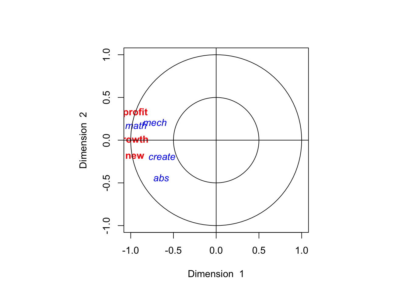
The following gives the correlation between the original variables and the transformed variables
##              [,1]          [,2]         [,3]
## growth -0.9798776  0.0006477883  0.199598477
## profit -0.9464085  0.3228847489 -0.007504408
## new -0.9518620 -0.1863009724 -0.243414776## [,1] [,2] [,3]
## create -0.6383313 -0.2156981 -0.65140953
## mech -0.7211626 0.2375644 0.06773775
## abs -0.6472493 -0.5013329 0.57422365
## math -0.9440859 0.1975329 0.09422619## [,1] [,2] [,3]
## growth -0.9744713 0.0005688272 0.076567107
## profit -0.9411869 0.2835272081 -0.002878734
## new -0.9466102 -0.1635921013 -0.093375287## [,1] [,2] [,3]
## create -0.6348095 -0.1894059 -0.24988439
## mech -0.7171837 0.2086069 0.02598458
## abs -0.6436782 -0.4402237 0.22027544
## math -0.9388771 0.1734549 0.03614570Describe the first pair of canonical variables, give their correlation, and provide an interpretation.
Describe the second pair of canonical variables, and provide an interpretation.
- Attempt exam question 1 part (b) from the 2017-18 exam paper.
Suppose that \(\bz = (\bx^\top \by^\top)^\top\) is a random vector, where both \(\bx\) and \(\by\) are sub-vectors of dimension \(p\), so that \(\bz\) is \((2p)\times 1\). Define \[\var(\bz)=\bSigma_{\bz \bz}=\begin{pmatrix} \bSigma_{\bx \bx} & \bSigma_{\bx \by}\\\bSigma_{\by \bx} & \bSigma_{\by \by} \end{pmatrix}.\]
- Suppose that \(\by = \bT \bx\) where \(\bT\) is a fixed matrix. Find \(\bSigma_{\bx \by}\) and \(\bSigma_{\by \by}\) in terms of \(\bSigma_{\bx \bx}\) and \(\bT\).
- Assuming now that \(\bT\) is an orthogonal matrix and \(\bSigma_{\bx \bx}\) is of full rank, determine the singular values of the matrix \(\bQ=\bSigma_{\bx \bx}^{-1/2}\bSigma_ {\bx \by}\bSigma_{\by \by}^{-1/2}\), and hence write down the canonical correlation coefficients.
- Suppose now that \(\bT\) is non-singular but not orthogonal. Comment on whether the answer to part (b) changes.
We will now prove Proposition ?? by induction. The case for \(k=1\) was proved in Section 3.1 in Proposition ??. Assume the result is true for \(k\). Consider the objective \[\mathcal{L} = \ba^\top \bQ \bb + \sum_{i=1}^k \gamma_i\ba^\top \ba_i + \sum_{i=1}^k \mu_i\bb^\top \bb_i + \frac{\lambda_1}{2}(1-\ba^\top\ba)+ \frac{\lambda_2}{2}(1-\bb^\top\bb)\] where \(\lambda_i, \mu_i, \gamma_i\) are Lagrangian multipliers.
By differentiating with respect to \(\ba\) and \(\bb\) and setting the derivative to zero show that \[\begin{align} \bQ\bb + \sum\gamma_i \ba_i - \lambda_1 \ba &= 0 \tag{3.1}\\ \bQ^\top\ba + \sum\mu_i \bb_i - \lambda_2 \bb &= 0. \tag{3.2} \end{align}\]
By left multiplying the equations above by \(\ba^\top\) and \(\bb^\top\) respectively show that \[\lambda_1=\lambda_2 = \ba^\top \bQ \bb.\]
By left multiplying (3.1) by \(\ba_i^\top\) show that \(\gamma_i=0\) for \(i=1, \ldots, k\). Show similarly that \(\mu_i =0\) for \(i=1, \ldots, k\).
Finally, by copying the proof of Proposition ??, prove Proposition ??.
Show the mean of the cc variables \(\eta_k\) and \(\psi_k\) is zero. Prove Proposition ?? giving the variance of covariance the cc variables.
Attempt exam question 1 part (b) from the 2020-21 exam paper.
- The
mtcarsdataset in R contains data on 32 cars from the 1970s. We will split the data into two datasets. Let \(\bX\) be the matrix that contains variables pertaining to car characteristics:
- cyl Number of cylinders
- disp Displacement (cu.in.)
- hp Gross horsepower
- drat Rear axle ratio
- wt Weight (1000 lbs)
and let \(\bY\) be the matrix containing variables pertaining to car performance:
- mpg Miles/(US) gallon
- qsec 1/4 mile time
We can then do CCA on these two datasets
## [1] 0.9270377 0.8307044## [,1] [,2]
## cyl -0.277988315 0.373120734
## disp 0.001628855 0.003177998
## hp -0.005964078 0.007770195
## drat 0.015934959 0.791032730
## wt -0.388097090 -1.423595709## [,1] [,2]
## mpg 0.1451984 0.1109009
## qsec 0.1346424 -0.6013371## [,1] [,2]
## cyl -0.9578700 0.07914027
## disp -0.9126296 -0.12094085
## hp -0.9164944 0.29160643
## drat 0.6666822 0.43010103
## wt -0.8643963 -0.47212540## [,1] [,2]
## mpg 0.9046387 0.1815048
## qsec 0.5627028 -0.6601685## [,1] [,2]
## cyl -0.8879817 0.06574217
## disp -0.8460421 -0.10046609
## hp -0.8496249 0.24223874
## drat 0.6180395 0.35728682
## wt -0.8013280 -0.39219665## [,1] [,2]
## mpg 0.9758380 0.2184951
## qsec 0.6069902 -0.7947093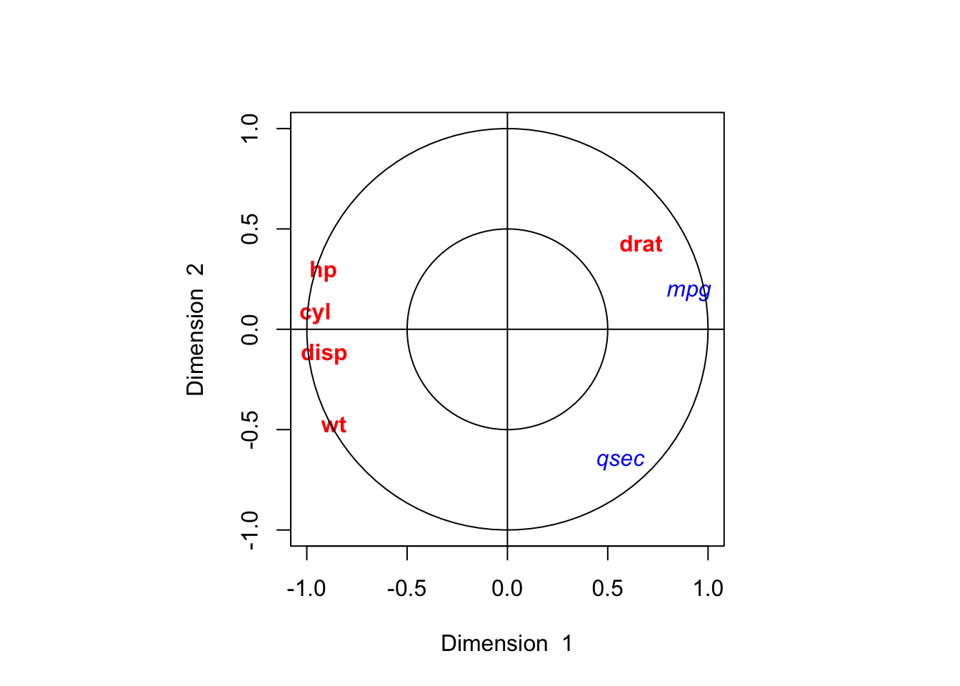
Interpret the output of this canonical correlation analysis.