1.1 Notation
We will think of datasets as consisting of measurements of \(p\) different variables for \(n\) different cases/subjects. We organise the data into an \(n \times p\) data matrix.
Multivariate analysis (MVA) refers to data analysis methods where there are two or more response variables for each case (you are familiar with situations where there is more than one explanatory variable, e.g., multiple linear regression).
We shall often write the data matrix as \(\mathbf X\) (\(n \times p\)) where \[ {\mathbf X}=\left[ \begin{array}{ccc} - &\mathbf x_1^\top&-\\ - &\mathbf x_2^\top&-\\ - &..&-\\ - &\mathbf x_n^\top&- \end{array}\right ] \] The vectors \(\mathbf x_1, \ldots , \mathbf x_n \in \mathbb{R}^p\) are the observation vectors for each of the \(n\) subjects.
- The \(n\) rows of \(\mathbf X\) are \(\mathbf x_1^\top, \ldots , \mathbf x_n^\top\) - each row contains the \(p\) observations on a single subject.
- The \(p\) columns of \(\mathbf X\) correspond to the \(p\) variables being measured, i.e., they contain the measurements of the same variable across all \(n\) subjects.
Important remark on notation: Throughout the module we shall use
- non-bold letters, whether upper or lower case, to indicate scalar (i.e. real-valued) quantities, e.g., \(x, y\)
- lower-case letters in bold to signify column vectors, e.g., \(\mathbf x, \mathbf y\)
- upper case letters in bold to signify matrices, e.g., \(\mathbf X, \mathbf Y\).
This convention for bold letters will also apply to random quantities. So, in particular, for a random vector we always use (bold) lower case, and for a random matrix we always use bold upper-case, regardless of whether we are referring to (i) the unobserved random quantity or (ii) its observed value. It should always be clear from the context which of these two interpretations (i) or (ii) is appropriate.
1.1.1 Example datasets
Example 1.1 The football league table is an example of multivariate data. Here \(W =\) number of wins, \(D =\) number of draws, \(F =\) number of goals scored and \(A =\) number of goals conceded for four teams. In this example we have \(p=4\) variables \((W, D, F, A)^\top\) measured on \(n=4\) cases (teams).
| Team | W | D | F | A |
|---|---|---|---|---|
| USA | 1 | 2 | 4 | 3 |
| England | 1 | 2 | 2 | 1 |
| Slovenia | 1 | 1 | 3 | 3 |
| Algeria | 0 | 1 | 0 | 2 |
The data vector for the USA is \[x_1^\top=(1,2,4,3)\]
Example 1.2 Exam marks for a set of \(n\) students where \(P =\) mark in probability and \(S =\) mark in statistics. Let \(x_{ij}\) denote the \(j\)th variable measured on the \(i\)th subject.
| Student | P | S |
|---|---|---|
| 1 | \(x_{11}\) | \(x_{12}\) |
| 2 | \(x_{21}\) | \(x_{22}\) |
| \(\vdots\) | \(\vdots\) | \(\vdots\) |
| n | \(x_{n1}\) | \(x_{n2}\) |
Example 1.3 The iris dataset is a famous set of measurements collected on the sepal length and width, and the petal length and width, of 50 flowers for each of 3 species of iris (setosa, versicolor, and virginica). The dataset is built into R (try typing iris in R) and is often used to demonstrate multivariate statistical methods. For these data, \(p=5\), and \(n=150\).
| Sepal.Length | Sepal.Width | Petal.Length | Petal.Width | Species |
|---|---|---|---|---|
| 5.1 | 3.5 | 1.4 | 0.2 | setosa |
| 4.9 | 3.0 | 1.4 | 0.2 | setosa |
| 4.7 | 3.2 | 1.3 | 0.2 | setosa |
| 7.0 | 3.2 | 4.7 | 1.4 | versicolor |
| 6.4 | 3.2 | 4.5 | 1.5 | versicolor |
| 6.9 | 3.1 | 4.9 | 1.5 | versicolor |
| 6.3 | 3.3 | 6.0 | 2.5 | virginica |
| 5.8 | 2.7 | 5.1 | 1.9 | virginica |
| 7.1 | 3.0 | 5.9 | 2.1 | virginica |
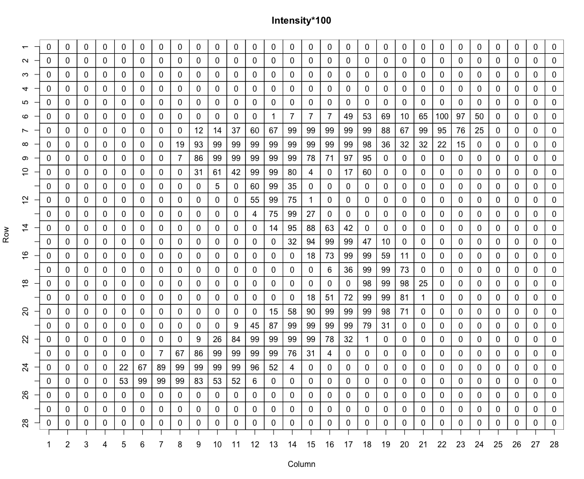
Example 1.4 The MNIST dataset is a collection of handwritten digits that is widely used in statistics and machine learning to test algorithms. It contains 60,000 images of hand-written digits. Here are the first 12 images:

Each digit has been converted to a grid of \(28\times 28\) pixels, with a grayscale intensity level specified for each pixel. When we store these on a computer, we flatten each grid to a vector of length 784. So for this dataset, \(n=60,000\) and \(p=784\). As an example of what the data look like, the intensities (times 100) for the first image above are shown in the plot below:
1.1.2 Aims of multivariate data analysis
The aim of multivariate statistical analysis is to answer questions such as:
- How can we visualise the data?
- What is the joint distribution of marks?
- Can we simplify the data? For example, we rank football teams using \(3W+D\) and we rank students by their average module mark. Is this fair? Can we reduce the dimension in a better way?
- Can we use the data to discriminate, for example, between male and female students?
- Are the different iris species different shapes?
- Can we build a model to predict the intended digit from an image of someones handwriting? Or predict the species of iris from measurements of its sepal and petal?
We could just apply standard univariate techniques to each variable in turn, but this ignores possible dependencies between the variables which we must represent to draw valid conclusions.
What is the difference between MVA and standard linear regression?
- In standard linear regression we have a scalar response variable, \(y\) say, and a vector of covariates, \(\mathbf x\), say. The focus of interest is on how knowledge of \(\mathbf x\) influences the distribution of \(y\) (in particular, the mean of \(y\)). In contrast, in MVA the focus is a vector \(\mathbf y\), in which all the components of \(\mathbf y\) are viewed as responses rather than covariates, possibly with additional covariate information \(\mathbf x\). We will discuss this further in Chapter 10.