8.2 Bayes discriminant rule
In the previous section, we implicitly assumed that each subject is equally likely to be from any of the \(g\) populations. This is the simplest case but is an unrealistic assumption in practice.
For example, suppose we want to classify photos on the internet as either being a photo of Bill Evans or not Bill Evans. Most photos on the internet are not of Bill Evans, and so we want to take this into account in the classifier, i.e., we want to take the base rate of occurence of each population into account.
Suppose a priori that the probability an observation is from population \(k\) is \(\pi_k\), with \[\sum_{k=1}^g \pi_k=1.\] Then given a probability model \(f_k(\mathbf x)\) for observations \(\mathbf x\) from population \(k\), our posterior probability for observation \(\mathbf x\) being from population \(k\) is \[{\mathbb{P}}(y=k \mid \mathbf x) = \frac{f_k(\mathbf x)\pi_k}{\sum_{j=1}^g f_j(\mathbf x)\pi_j}\] by Bayes theorem.
Definition 8.2 The Bayes classifier assigns \(\mathbf x\) to the population for which the posterior probability is highest: \[d^{Bayes}(\mathbf x) =\arg \max_k {\mathbb{P}}(y=k \mid \mathbf x).\]
As before, if we assume each population has a multivariate normal distribution, then this simplifies.
Proposition 8.3 If cases in population \(\Pi_k\) have a \(N_p({\boldsymbol{\mu}}_k,\boldsymbol{\Sigma})\) distribution, then the Bayes discriminant rule is \[d(\mathbf x)= \arg\min_{k} \frac{1}{2}(\mathbf x-{\boldsymbol{\mu}}_k)^\top \boldsymbol{\Sigma}^{-1} (\mathbf x-{\boldsymbol{\mu}}_k)- \log \pi_k.\]
Equivalently, if \[\delta_k(\mathbf x) = {\boldsymbol{\mu}}_k^\top \boldsymbol{\Sigma}^{-1} \mathbf x-\frac{1}{2}{\boldsymbol{\mu}}_k^\top \Sigma^{-1} {\boldsymbol{\mu}}_k +\log \pi_k\] then \[d(\mathbf x) = \arg \max \delta_k(\mathbf x).\] I.e. this is a linear discriminant rule.
Proof. See the exercises.
Note that if \(\pi_k=\frac{1}{g}\) for all \(k\), then we can ignore \(\pi_k\) in the maximization, and the Bayes discriminant rule is exactly the same as the ML discriminant rule.
For two populations, the Bayes analogue of Corollary 8.1 is that we classify \(\mathbf x\) to population 1 if \[\mathbf a^\top(\mathbf x-\mathbf h)> \log\frac{\pi_2}{\pi_1}.\] The effect of the prior probabilities on the populations is to shift the decision boundary to be further away from the more likely class. For example, if in Example 2 we had \(\pi_1 = 0.9\) and \(\pi_2=0.1\) we get the decision boundary at \(x_1 = -2.19722\) as shown in Figure 8.5.
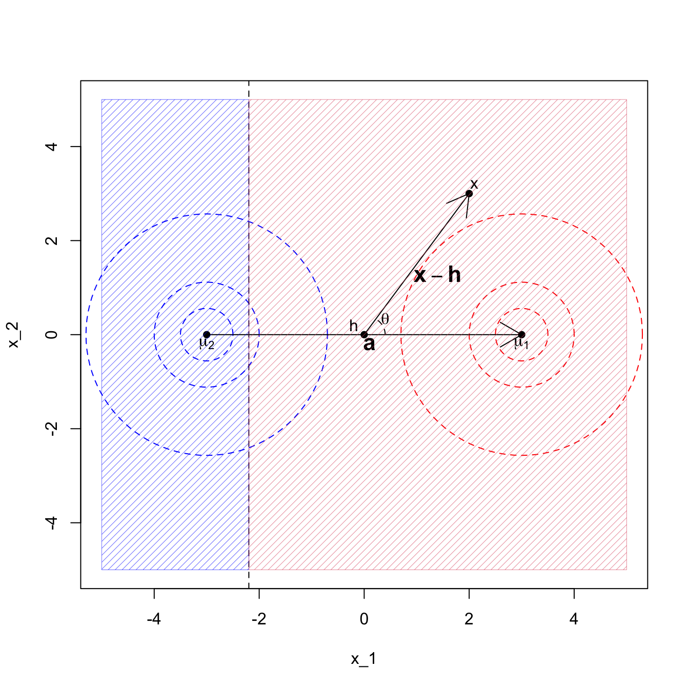
Figure 8.5: LDA when the covariance matrix is the identity, with class prior pi1=0.9
In practice, we may not know the population probabilities \(\pi_k\). If so, we can estimate them from the data using \[\hat{\pi}_k = \frac{n_k}{n}\] and substitute \(\hat{\pi}_k\) for \(\pi_k\) (as well as substituting \(\hat{{\boldsymbol{\mu}}}_k\), \(\widehat{\boldsymbol{\Sigma}}\) etc).
The lda command from the MASS library uses the Bayes discriminant rule, but gives you the option of setting \(\pi_k\) if known, but otherwise estimates the class probabilities.
8.2.1 Example: LDA using the Iris data
Let’s consider doing LDA with the iris data. To begin with, lets use just the setosa and virginica species so that we only have \(g=2\) populations, \(\Pi_{setosa}\) and \(\Pi_{virginica}\). We will also just use the sepal measurements so that \(p=2\). If we plot the data, we can see that the two populations should be easy to classify using just these two measurements:

The sample means and variances for each group are
\[\begin{eqnarray*} \hat{{\boldsymbol{\mu}}}_s = \begin{pmatrix}5.01 \\3.43 \\\end{pmatrix} &\qquad& \hat{{\boldsymbol{\mu}}}_v = \begin{pmatrix}6.59 \\2.97 \\\end{pmatrix} \\ \mathbf S_s = \begin{pmatrix}0.124&0.0992 \\0.0992&0.144 \\\end{pmatrix} &\qquad& \mathbf S_v =\begin{pmatrix}0.404&0.0938 \\0.0938&0.104 \\\end{pmatrix} \end{eqnarray*}\] where the \(s\) subscript gives the values for setosa, and \(v\) for virginica.
We have data on \(n=50\) flowers in each population. Hence, \[\begin{eqnarray*} \widehat{\boldsymbol{\Sigma}} &=& \frac{1}{50+50-2} \left(50 \mathbf S_s + 50 \mathbf S_v \right)= \begin{pmatrix}0.27&0.0985 \\0.0985&0.126 \\\end{pmatrix}, \\ \hat{{\boldsymbol{\mu}}}_s - \hat{{\boldsymbol{\mu}}}_v &=& \begin{pmatrix}-1.58 \\0.454 \\\end{pmatrix}, \\ \hat{\mathbf h} &=& \frac{1}{2} (\hat{{\boldsymbol{\mu}}}_s + \hat{{\boldsymbol{\mu}}}_v) = \begin{pmatrix}5.797 \\3.201 \\\end{pmatrix}, \end{eqnarray*}\] and \[\hat{\mathbf a} = \widehat{\boldsymbol{\Sigma}}^{-1} (\hat{{\boldsymbol{\mu}}}_s - \hat{{\boldsymbol{\mu}}}_v) = \begin{pmatrix}5.18&-4.04 \\-4.04&11.1 \\\end{pmatrix} \begin{pmatrix}-1.58 \\0.454 \\\end{pmatrix} = \begin{pmatrix}-10.031 \\11.407 \\\end{pmatrix}.\]
We can find these values in R as follows:
library(dplyr)
# select two measurements and two species
iris3 <- iris %>% dplyr::filter(Species != "versicolor") %>%
  dplyr::select(Sepal.Length, Sepal.Width, Species)

S_vir = iris3 %>% dplyr::filter(Species=="virginica") %>%
  dplyr::select(Sepal.Length, Sepal.Width) %>%
  cov
S_set = iris3 %>% dplyr::filter(Species=="setosa") %>%
  dplyr::select(Sepal.Length, Sepal.Width) %>%
  cov
S_u = (50*S_vir+50*S_set)/98


# Or more easily using a package
library(vcvComp)
S_u = cov.W(iris3[,1:2], iris3[,3])
The sample ML discriminant rule allocates a new observation \(\mathbf x= (x_1, x_2)^\top\) to \(\Pi_{\mbox{setosa}}\) if and only if \[ \hat{\mathbf a}^\top (\mathbf x- \hat{\mathbf h}) = \begin{pmatrix}-10.031&11.407 \\\end{pmatrix} \begin{pmatrix} x_1 - 5.797 \\ x_2 - 3.201 \end{pmatrix} > 0.\]
If we draw on the line defined by \[\mathbf a^\top (\mathbf x-\mathbf h)=0\] which can be written as \[x_2 = \frac{1}{a_2}(\mathbf a^\top\mathbf h-a_1x_1) = -1.8963517 - -0.8793085 x_1\] we can see this line clearly separates the two species of iris.
## Warning in geom_point(mapping = aes(x = 5.8, y = 2.5), color = "black", : All aesthetics have length 1, but the data has 100 rows.
## ℹ Please consider using `annotate()` or provide this layer with data containing
##   a single row.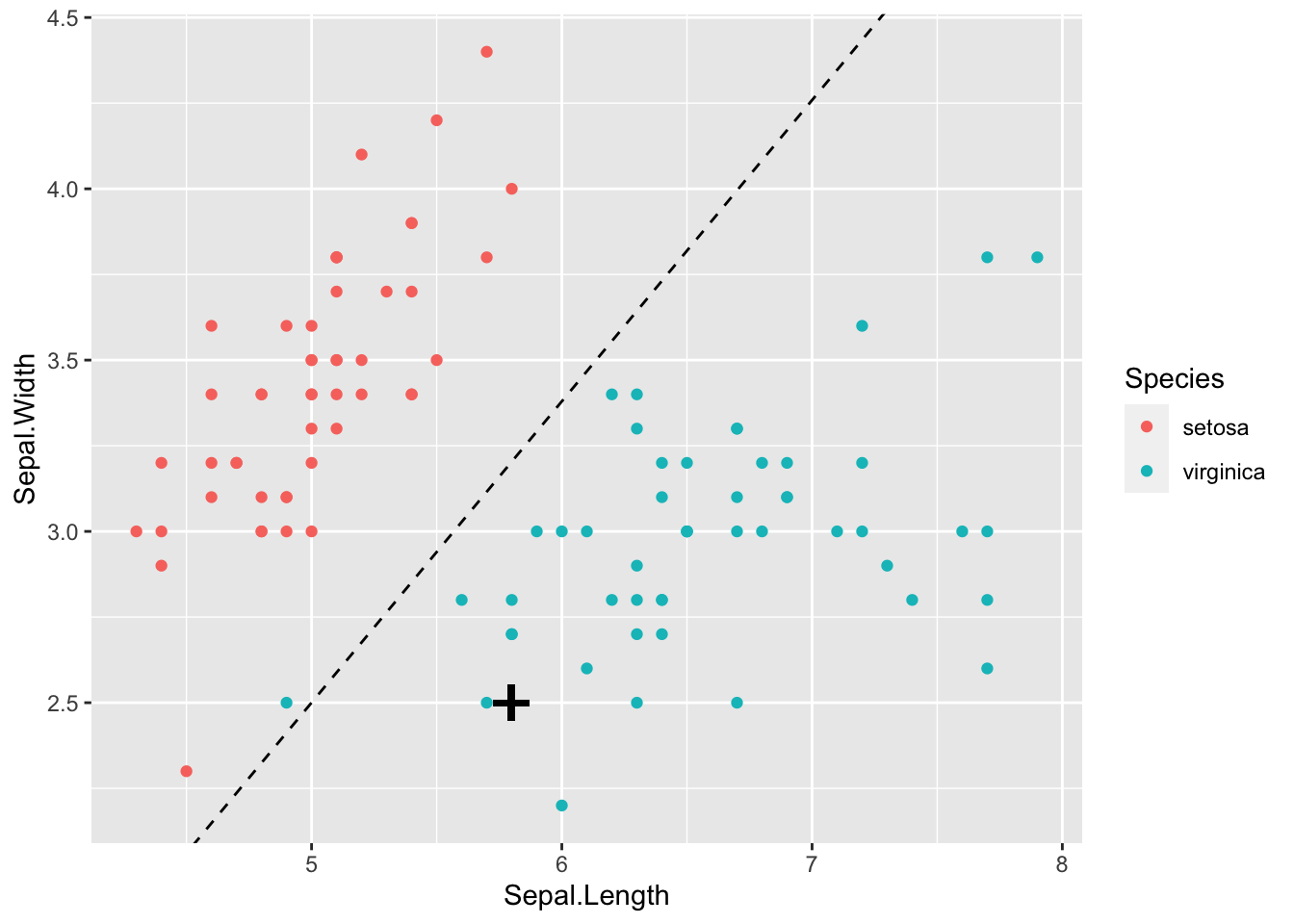
If a new iris had a sepal length of 5.8 and a sepal width of 2.5 (marked as a black cross on the plot above) then
\[ \hat{\mathbf a}^\top (\mathbf x- \hat{\mathbf h}) = \begin{pmatrix}-10.031&11.407 \\\end{pmatrix} \begin{pmatrix} 5.8 - 5.797 \\ 2.5 - 3.201 \end{pmatrix} =-8.0267032 < 0,\] and so we would allocate this iris to the virginia population, \(\Pi_{virginica}\).
As you would expect, there is an R command to do this for us: lda (for Linear Discriminant Analysis). This is in the MASS R package.
library(MASS)
iris.lda1 <- lda(Species ~ ., iris3)

# lda(Species ~ Sepal.Length+Sepal.Width, iris3)
  #  does the same thing
iris.lda1
## Call:
## lda(Species ~ ., data = iris3)
##
## Prior probabilities of groups:
## setosa virginica
## 0.5 0.5
##
## Group means:
## Sepal.Length Sepal.Width
## setosa 5.006 3.428
## virginica 6.588 2.974
##
## Coefficients of linear discriminants:
## LD1
## Sepal.Length 2.208596
## Sepal.Width -2.511742You can see that this has printed the group means, and the lda coefficients. The coefficients are different to the ones we computed for \(\mathbf a\), but have the same ratio, which is all that matters (because the discriminant planes are perpendicular to \(\mathbf a\) - multiplying \(\mathbf a\) by a constant does not change the plane).
The output also includes estimates of the prior probabilities for the two species, which are estimated to be \[\hat{\pi}_s = \frac{1}{2}, \quad \hat{\pi}_v = \frac{1}{2}\] as there were 50 irises from each population in the training data.
We can use the predict command to predict the species for a new observation \(\mathbf x\). Using the example from before of an iris with a sepal length of 5.8 and a sepal width of 2.5 we find the Bayes classifier predicts this is a virginica iris.
## $class
## [1] virginica
## Levels: setosa versicolor virginica
##
## $posterior
##         setosa virginica
## 1 0.0002771946 0.9997228
##
## $x
##        LD1
## 1 1.767357
Note that we are also given estimates of the probability that \(\mathbf x\) lies in each of the populations. These are computed using \[\frac{f_k(\mathbf x)\pi_k}{\sum_{j=1}^g f_j(\mathbf x)\pi_j}\] with the parameter estimates substituted for the unknown parameters.
Using the entire dataset
Let’s now use all 150 observations (with three populations: setosa, virginica, versicolor), and all four measurements.
## Call:
## lda(Species ~ ., data = iris)
##
## Prior probabilities of groups:
##     setosa versicolor  virginica
##  0.3333333  0.3333333  0.3333333
##
## Group means:
##            Sepal.Length Sepal.Width Petal.Length Petal.Width
## setosa            5.006       3.428        1.462       0.246
## versicolor        5.936       2.770        4.260       1.326
## virginica         6.588       2.974        5.552       2.026
##
## Coefficients of linear discriminants:
##                     LD1         LD2
## Sepal.Length  0.8293776 -0.02410215
## Sepal.Width   1.5344731 -2.16452123
## Petal.Length -2.2012117  0.93192121
## Petal.Width  -2.8104603 -2.83918785
##
## Proportion of trace:
##    LD1    LD2
## 0.9912 0.0088
We will delay discussion of what the reported coefficients mean, and how to visualize LDA, until after we have seen Fisher’s linear discriminant analysis in the next section. But we can use the klaR package to visualize a little of what LDA does. The partimat command provides an array of figures that show the discriminant regions based on every combination of two variables (i.e., it does LDA for each pair of variables).
library(klaR)
library(plyr)
Species_new= revalue(iris$Species, c("versicolor"="color"))

partimat(Species_new ~ Sepal.Length + Sepal.Width + Petal.Length
         + Petal.Width,
         data=iris, method="lda")
Note that I renamed the versicolor species as color so that the different species appear more clearly in the plots.
8.2.2 Quadratic Discriminant Analysis (QDA)
We have seen that in the case where the populations all share a common covariance matrix, \(\boldsymbol{\Sigma}\), that the decision boundaries are linear (i.e., hyperplanes). We also saw in example 8.2 in a one-dimensional example that when the two populations had different variances we have a quadratic decision boundary.
In general, if we allow the variances to differ between populations, so that we model population \(k\) as \[\mathbf x\sim N_p({\boldsymbol{\mu}}_k, \boldsymbol{\Sigma}_k),\] then we get the Bayes discriminant rule \[ d(\mathbf x)=\arg\max_k \left(-\frac{1}{2} \log |\boldsymbol{\Sigma}_k| - \frac{1}{2}(\mathbf x-{\boldsymbol{\mu}}_k)^\top \boldsymbol{\Sigma}_k^{-1} (\mathbf x-{\boldsymbol{\mu}}_k)+\log \pi_k\right). \]
We can not ignore the quadratic term in \(\mathbf x\) as it depends upon the population indicator \(k\). We also have to include the determinant of \(\boldsymbol{\Sigma}_k\). Thus in this case we get a quadratic decision boundary rather than a linear one.
8.2.2.1 Iris example continued
The qda function in the MASS package implements quadratic discriminant analysis.
We can again use the partimat command to look at the decision boundaries if we do QDA for each pair of variables in turn.
partimat(Species ~ Sepal.Length + Sepal.Width + Petal.Length +
           Petal.Width,         data=iris, method="qda")
8.2.3 Prediction accuracy
To assess the predictive accuracy of our discriminant rules, we often split the data into two parts, a training set, and a test set. Let’s do this randomly by chosing 100 of the irises to be in our training set, and use the other 50 irises in the test set. We will then train the classifiers on the training set, and predict the species labels for test dataset. We can then count how many predictions were correct.
set.seed(2)
test.ind <- sample(150, size=50)
iris.test <- iris[test.ind,]
iris.train <- iris[-test.ind,]

lda1 <- lda(Species~., iris.train)
qda1 <- qda(Species~., iris.train)
test.ldapred <- predict(lda1, iris.test)
test.qdapred <- predict(qda1, iris.test)
(lda.accuracy <- sum(test.ldapred$class==iris.test$Species))/50
## [1] 0.98## [1] 0.98So in this case we find that LDA and QDA both have an accuracy of 4900%, which is the result of a single wrong prediction. We can see more clearly what has gone wrong by using the table command.
##
##              setosa versicolor virginica
##   setosa         17          0         0
##   versicolor      0         15         0
##   virginica       0          1        17
These tables of results are known as confusion matrices.
So in this case one of the virginica irises was predicted incorrectly to be versicolor.
Here we randomly split the data into test and training sets. With small datasets such as this (\(n=150\)), we instead sometimes use cross validation to assess the accuracy of each method. To do this, we split the data up into test and training sets multiple times randomly, and assess the prediction error on each random split.