4.5 Exercises
- Consider the following data in \(\mathbb{R}^2\)
\[\mathbf x_1 =\begin{pmatrix}1\\-1\end{pmatrix},\; \mathbf x_2 =\begin{pmatrix}-1\\1\end{pmatrix}, \;\mathbf x_3 =\begin{pmatrix}2\\2\end{pmatrix}\]
What is the orthogonal projection of these points onto \[\mathbf u_1 = \begin{pmatrix}1\\0\end{pmatrix}\] and onto \[\mathbf u_2 =\frac{1}{\sqrt{5}}\begin{pmatrix}1\\2\end{pmatrix}?\]
Compute the sample variance matrix of the data points, and compute its spectral decomposition.
Which unit vector \(\mathbf u\) would maximize the variance of these projections?
What vector \(\mathbf u\) would minimize \[\sum_{i=1}^4 ||\mathbf x_i -\mathbf u\mathbf u^\top \mathbf x_i||^2_2?\] This is the sum of squared errors from a rank 1 approximation to the data.
Plot the data points and convince yourself that your answers make intuitive sense.
- Consider a population covariance matrix \(\boldsymbol{\Sigma}\) of the form
\[\boldsymbol{\Sigma}=\gamma \mathbf I_p + \mathbf a\mathbf a^\top\]
where \(\gamma>0\) is a scalar, \(\mathbf I_p\) is the \(p \times p\) identity matrix and \(\mathbf a\) is a vector of dimension \(p\).
- Show that \(\mathbf a\) is an eigenvector of \(\boldsymbol{\Sigma}\).
- Show that if \(\mathbf b\) is any vector such that \(\mathbf a^\top \mathbf b=0\), then \(\mathbf b\) is also an eigenvector of \(\boldsymbol{\Sigma}\). What is the eigenvalue corresponding to \(\mathbf b\)?
- Obtain all the eigenvalues of \(\boldsymbol{\Sigma}\).
- Determine expressions for the proportion of variability ‘explained’ by:
- the largest (population) principal component of \(\boldsymbol{\Sigma}\);
- the \(r\) largest (population) principal components of \(\boldsymbol{\Sigma}\), where \(1 < r \leq p\).
- A covariance matrix has the following eigenvalues:
## [1] 4.22 2.38 1.88 1.11 0.91 0.82 0.58 0.44 0.35 0.19 0.05 0.04 0.04- Sketch a scree plot.
- Determine the minimum number of principal components needed to explain 90% of the total variation.
- Determine the number of principal components whose eigenvalues are above average.
Measurements are taken on \(p=3\) variables \(x_1\), \(x_2\) and \(x_3\), with sample correlation matrix \[ \mathbf R= \begin{pmatrix} 1 & 0.5792 & 0.2414 \\ 0.5792 & 1 & 0.5816 \\ 0.2414 & 0.5816 & 1 \end{pmatrix}. \] The variable \(z_j\) is the standardised versions of \(x_j\), \(j=1,2,3\), i.e. each \(z_j\) has sample mean \(0\) and variance \(1\). One observation has \(z_1 = z_2 = z_3 = 0\) and a second observation has \(z_1 = z_2 = z_3 =1\). Calculate the three principal component scores for each of these observations.
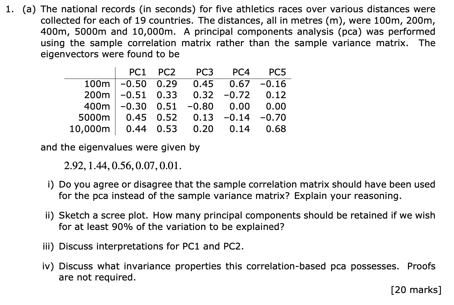
Try exam question 1 part (a) from the 2017-18 exam paper.
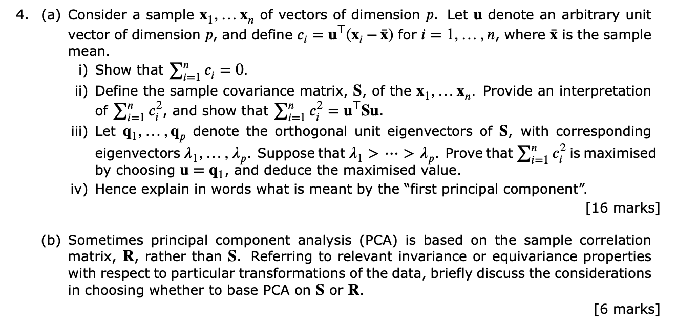
- This is an exam question from 2019.
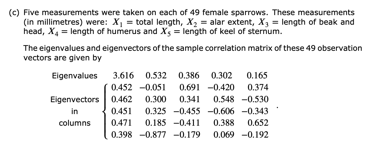
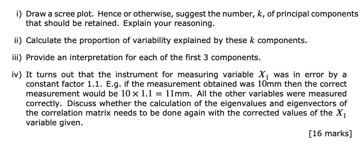
- Try this tricky question from the 2016 exam.