Chapter 6 Multidimensional Scaling (MDS)
The videos for this chapter are available at:
- 6.0 Introduction to MDS
- 6.1 Classical MDS
- 6.1 Example 1
- 6.1.1 Non-Euclidean distance matrices
- 6.1.2 Principal Coordinate Analysis
- 6.2 Similarity measures
- 6.2.1 Binary attributes
- 6.3 Non-metric MDS
In PCA, we start with \(n\) data points \(\mathbf x_i \in \mathbb{R}^p\), and then try to find a low dimensional projection of these points, e.g., \(\mathbf y_1, \ldots, \mathbf y_n \in \mathbb{R}^r\) with \(r<p\), in such a way that they minimize the reconstruction error (or maximize the variance).
The focus in Multidimensional Scaling (MDS) is somewhat different. Instead of being given the data \(\mathbf X\), our starting point is often a matrix of distances or dissimilarities between the data points, \(\mathbf D\). For example, if we have data on \(n\) different experimental units, then we would be given the distances \(d_{ij}\) between any pair of experimental units \(i\) and \(j\). We compile these into a \(n\times n\) distance matrix \(\mathbf D=(d_{ij}: \, i,j=1, \ldots , n)\).
The goal of MDS is to find a set of points in a low-dimensional Euclidean space \(\mathbb{R}^r\), usually \(\mathbb{R}\) or \(\mathbb{R}^2\), whose inter-point distances (or dissimilarities) are as close as possible to the \(d_{ij}\). That is, we want to find \(\mathbf y_1, \ldots, \mathbf y_n \in \mathbb{R}^r\) whose distance matrix is approximately \(\mathbf D\), i.e., for which \[\operatorname{distance}(\mathbf y_i, \mathbf y_j) \approx d_{ij}.\] In other words, we are trying to create a spatial representation of the data, \(\mathbf y_1, \ldots, \mathbf y_n\), from a distance matrix \(\mathbf D\). The vectors \(\mathbf y_i\) have no meaning by themselves, but by visualising their spatial pattern we can hope to learn something about the dataset represented by \(\mathbf D\).
If we define the errors in terms of a square distance, then we can write the goal of MDS as the following optimization problem: \[\begin{align} \mbox{Find} \quad& \mathbf y_1, \ldots, \mathbf y_n \in \mathbb{R}^r\\ \mbox{to minimize} \quad &\sum_{i=1}^n \sum_{j=1}^n (d_{ij} - d(\mathbf y_i, \mathbf y_j))^2.\tag{6.1} \end{align}\]
As an illustrative example, consider the location of some of England’s cities.
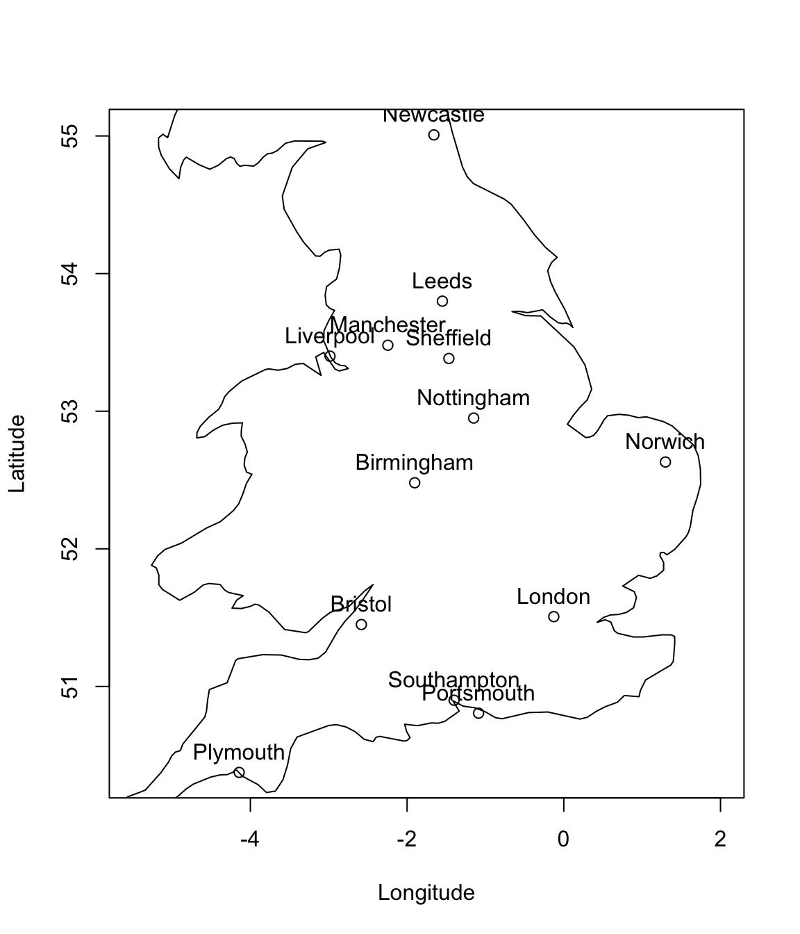
If we are told their latitude and longitude, it is easy to calculate the distances between the cities. I.e., given the latitude and longitude of each city, \(\mathbf x_i\), we can compute the distance matrix between pairs of cities \(\mathbf D\):
| London | Birmingham | Manchester | Leeds | Newcastle | Liverpool | Portsmouth | Southampton | Nottingham | Bristol | Sheffield | Norwich | Plymouth | |
|---|---|---|---|---|---|---|---|---|---|---|---|---|---|
| London | 0 | 163 | 262 | 273 | 403 | 286 | 103 | 112 | 175 | 170 | 228 | 159 | 308 |
| Birmingham | 163 | 0 | 114 | 149 | 282 | 125 | 195 | 179 | 73 | 124 | 105 | 217 | 281 |
| Manchester | 262 | 114 | 0 | 58 | 174 | 50 | 308 | 293 | 94 | 227 | 53 | 255 | 369 |
| Leeds | 273 | 149 | 58 | 0 | 135 | 105 | 335 | 323 | 98 | 271 | 47 | 230 | 420 |
| Newcastle | 403 | 282 | 174 | 135 | 0 | 199 | 469 | 458 | 231 | 401 | 181 | 328 | 542 |
| Liverpool | 286 | 125 | 50 | 105 | 199 | 0 | 317 | 299 | 132 | 219 | 101 | 299 | 346 |
| Portsmouth | 103 | 195 | 308 | 335 | 469 | 317 | 0 | 24 | 239 | 127 | 288 | 261 | 221 |
| Southampton | 112 | 179 | 293 | 323 | 458 | 299 | 24 | 0 | 229 | 103 | 276 | 268 | 202 |
| Nottingham | 175 | 73 | 94 | 98 | 231 | 132 | 239 | 229 | 0 | 193 | 53 | 169 | 353 |
| Bristol | 170 | 124 | 227 | 271 | 401 | 219 | 127 | 103 | 193 | 0 | 228 | 296 | 162 |
| Sheffield | 228 | 105 | 53 | 47 | 181 | 101 | 288 | 276 | 53 | 228 | 0 | 203 | 382 |
| Norwich | 159 | 217 | 255 | 230 | 328 | 299 | 261 | 268 | 169 | 296 | 203 | 0 | 453 |
| Plymouth | 308 | 281 | 369 | 420 | 542 | 346 | 221 | 202 | 353 | 162 | 382 | 453 | 0 |
But can we do the reverse and construct a map from the distance matrix? This is the aim of multidimensional scaling: MDS constructs a set of points, \(\mathbf y_1, \ldots, \mathbf y_n\), that have distances between them given by the distance matrix \(\mathbf D\). In other words, it creates a map with a set of coordinates for which the distances between points are approximately the same as in the real data.
Of course, this illustrative example is not very interesting, as the original data (the city locations) are only two-dimensional, but in problems with high dimensional data, finding a way to represent the points in a low-dimensional space will make visualization and statistical analysis easier. We shall see, perhaps unsurprisingly, that there is a close connection between MDS and PCA.
Notation
There are many ways to compute distances between points. For example, you may have studied metrics previously, which are distance functions that satisfy certain axioms. In MDS, we do not need to work with distances that are metrics (although sometimes we do), and instead we only require that distances satisfy a weaker set of conditions:
Definition 6.1 The \(n \times n\) matrix \(\mathbf D=(d_{ij})_{i,j=1}^n\) is a distance matrix (sometimes called a dissimilarity matrix) if
- \(d_{ij}\geq 0\) for all \(i, j=1,\ldots,n\).
- \(d_{ii}=0\) for \(i=1,\ldots, n\) and
- \(\mathbf D=\mathbf D^\top\), i.e., \(\mathbf D\) is symmetric (\(d_{ij}=d_{ji}\)).
Note that we do not require distances to necessarily satisfy the triangle inequality \[\begin{equation} d_{ik} \leq d_{ij}+d_{jk}. \tag{6.2} \end{equation}\] A distance function which always satisfies the triangle inequality is called a metric distance or just a metric. A distance function which does not always satisfy the triangle inequality is called a non-metric distance.
There are many ways to measure distance. Two common choices of metric distances are
- Euclidean distance \(||\mathbf x-\mathbf x'||_2\), also know as the ‘crow flies’ distance.
- \(L_1\) distance \(||\mathbf x-\mathbf x'||_1\), sometimes called the Manhattan or taxicab metric.
But for the city data, we could also consider distance by road, i.e., we could measure the minimum distance by road between each pair of cities. This would satisfy the axioms for being a distance, but is not a metric distance
The choice of which distance is appropriate is problem specific (see section 6.2 for an example). The focus in this chapter is on Euclidean distance, as this leads to an explicit mathematical solution to the optimization problem (6.1). However, note that MDS techniques have also been developed for non-Euclidean distances.