Chapter 8 Discriminant analysis

The videos for this chapter are available at the links below:

• Introduction
• Maximum likelihood discriminant rule
• Two populations
• Bayes discriminant rule
• Example: Iris data
• Fisher’s LDA
  
• Iris example revisited + links to other methods

We consider the situation in which there are \(g\) populations/classes \(\Pi_1, \ldots , \Pi_g\). Each subject/case belongs to precisely one population. For example

• for the iris data the populations are the 3 species {Setosa, Versicolor, Viriginica}. Each iris has a single species label.

• for the MNIST data, the populations are the digits 0 to 9. Each image represents a single digit.

Suppose we are given measurements \(\mathbf x_i\) on each subject, and population/class label \(y_i\). The aim of classification is to build a model to predict the class label \(y\) from a set of measurements \(\mathbf x\). For our examples:

• iris: the measurements \(\mathbf x_i\in \mathbb{R}^{4}\) are the sepal and petal width and lengths. The class label \(y_i\) is the species.

• mnist: \(\mathbf x_i\in \mathbb{R}^{784}\) is a vector of pixel intensities. The class label \(y_i\) is the digit the image represents.

If \(\mathbf x\in \mathbb R^p\) is a ‘new’ observation assumed to come from one of \(\Pi_1, \ldots , \Pi_g\), the aim of discriminant analysis is to allocate \(\mathbf x\) to one of \(\Pi_1, \ldots , \Pi_g\) with as small a probability of error as possible.

A discriminant rule, \(d\), corresponds to a partition of \(\mathbb R^p\) into disjoint regions \(\mathcal R_1, \ldots, \mathcal R_g\), where \[\bigcup_{j=1}^g \mathcal R_j = \mathbb R^p, \qquad \mathcal R_j \cap \mathcal R_k = \emptyset, j \neq k.\] The rule \(d\) is then defined by

\(d\): allocate \(\mathbf x\) to \(\Pi_j\) if and only if \(\mathbf x\in \mathcal R_j\).

The way we find a rule \(d\), is by defining discriminant functions, \(\delta_j(\mathbf x)\), for each population \(j=1, \ldots, g\). We classify \(\mathbf x\) to population \(j\) if \(\delta_j(\mathbf x)>\delta_i(\mathbf x)\) for \(i \not = j\). We can write this as

\[d(\mathbf x) = \arg \max_j \delta_j(\mathbf x),\] i.e., \(d\) is a map from \(\mathbb{R}^p\) to \(\{1, \ldots, g\}\)

Linear discriminant analysis

We will focus on discriminant functions that are affine functions of the data. That is they are linear projections of the data plus a constant of the form \[\begin{equation} \delta_j(\mathbf x) = \mathbf v_j^\top \mathbf x+ c_j. \tag{8.1} \end{equation}\]

In later sections we will discuss how to choose the discriminant rules \(\delta_j(\mathbf x)\), i.e., how to choose the parameters \(\mathbf v_j\) and \(c_j\). But first we focus on what the discriminant regions look like and how to classify points given a discriminant rule.

Geometry of LDA

Proposition 8.1 The discriminant regions \(\mathcal{R}_j\) corresponding to affine discriminant functions are convex and connected.

Proof. You will prove this in the exercises.

Recall that the equation of a hyperplane of dimension \(p-1\) in \(\mathbb{R}^p\) requires us to specify a point on the plane, \(\mathbf x_0\), and a vector from the origin that is perpendicular/orthogonal to the plane, \(\mathbf n\). The hyperplane can then be described as \[ \mathcal{H}(\mathbf n, \mathbf x_0) =\{\mathbf x\in \mathbb{R}^p:\, \mathbf n^\top (\mathbf x-\mathbf x_0) =0\} \]

The orthogonal distance from the origin to the plane is \[\frac{1}{||\mathbf n||}\mathbf x_0^\top \mathbf n.\]

Affine discriminant functions (8.1) divide \(\mathbb{R}^p\) into regions using \((p-1)\)-dimensional hyperplanes, which results in decision regions that have linear boundaries.

To see this, consider the cases where there are just two populations (\(g=2\)). We classify a point \(\mathbf x\) as population 1 if \(\delta_1(\mathbf x) > \delta_2(\mathbf x)\), and the decision boundary is at \[\delta_1(\mathbf x) = \delta_2(\mathbf x).\]

If \(\mathbf x\) is on the decision boundary then

\[(\mathbf v_1-\mathbf v_2)^\top \mathbf x+ c_1 -c_2=0.\] This can be seen to be the equation of a hyperplane with normal vector \(\mathbf v_1-\mathbf v_2\). The orthogonal distance of the plane from the origin is \[\frac{|c_2-c_1|}{||\mathbf v_1-\mathbf v_2||}.\]

Example 8.1 Let’s consider the case of 3 populations with data in \(\mathbb{R}^2\). Suppose the discriminant functions have

\[\mathbf v_1 = \begin{pmatrix}1\\1\end{pmatrix}, \quad \mathbf v_2 = \begin{pmatrix}2\\0\end{pmatrix}, \quad\mathbf v_3 = \begin{pmatrix}1\\-1\end{pmatrix}\] and \[c_1=1, \quad c_2=-1, \quad c_3=0.\]

Then

• the decision boundary between population 1 and 2 is the line with equation \[y=x-2\] and has orthogonal distance \(\sqrt{2}\) from the origin;

• the decision boundary between population 1 and 3 is the line with equation \[y=-\frac{1}{2}\] which has orthogonal distance \(\frac{1}{2}\) from the origin;

• the decision boundary between population 2 and 3 is the line with equation \[y=-x+1.\] which has orthogonal distance \(\frac{1}{\sqrt{2}}\) from the origin.

If we plot these, then you can see that this results in the decision regions shown in Figure 8.1.

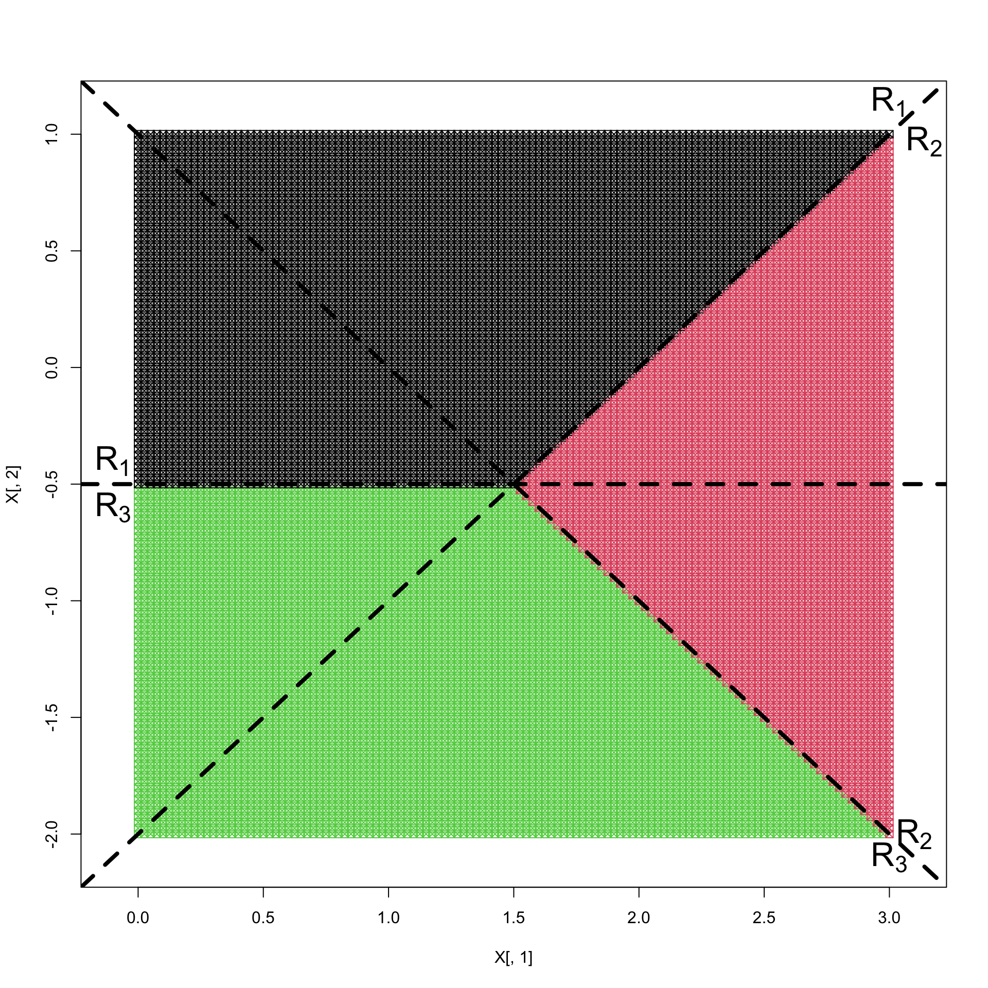
Figure 8.1: Discriminant regions for Example 1.

In the following sections we consider several different approaches to deciding upon a suitable choice of \(\mathbf v_j\) and \(c_j\) in Equation (8.1).

1. By assuming the populations have a multivariate normal distribution. This is the focus of section 8.1, where we assume each population is equally likely. We generalise this approach in Section 8.2 to consider the situation where observations are more likely to be some from populations than from others.

2. By looking for linear projections of the data that maximize the spread between the different populations, i.e., that are best for distinguishing between different populations. This leads to Fisher’s discriminant rule which we cover in Section 8.3, and it does not require us to make assumptions about the distribution of the underlying populations.